
Overview
- This article will introduce new features in Excel.
What’s new ?
- Excel 2016 makes it easy to handle figures. With Excel 2016, you can streamline data entry using the AutoFill feature. Then, get the recommended charts based on your data and create the chart with a click of a button. Or easily detect trends and styles thanks to data columns, color codes, and icons.
Excel 2016 quick start features:
Insert information:
- To enter data manually:
- Select a blank cell, like A1, and then enter text or a number.
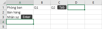
- Press Enter or Tab to move to the next cell.
- To enter the data series:
- Enter the beginning of the string into two cells: Jan and Feb; or 2014 and 2015.

- Select the two cells that contain the series, and then drag the fill handle over or down to the cells.
Fill column data with the AutoComplete feature with Preview:
Use the AutoComplete with Preview feature to automatically populate a column, such as Name, derived from another column, such as Full Name.
- In the box below Name, type Molly and press Enter.
- In the next box, enter the first few letters of Garret.
- When the list of suggested values appears, press Back.
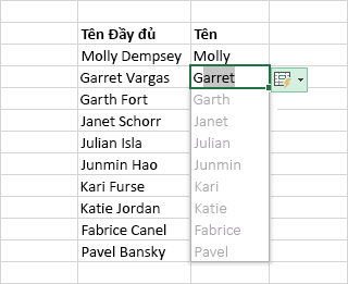
- Select AutoComplete Options with Preview to perform more operations.
Quick calculation with AutoSum feature:
- Select the box below the numbers you want to add.
- Select Home > AutoSum (in the Editing group).
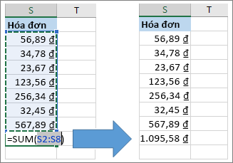
- In the selected box, press Back to see the result.
- To perform other calculations, select Home, select the down arrow next to AutoSum, and then select a calculation.
Create the chart:
Easily select the appropriate chart for your data with the Quick Analysis tool.
- Select the range of data you want to display in the chart.
- Select the Quick Analysis button in the lower right corner of the collection.
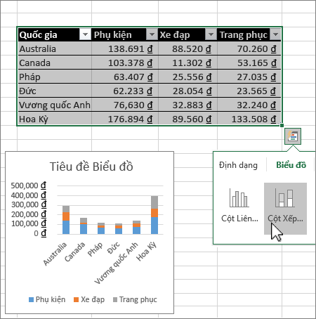
- Select Chart, hover over each proposed chart, then select the chart you like, such as Stacking.
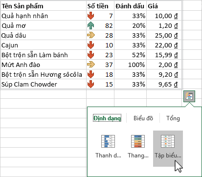
Use conditional formatting:
Highlight important data or show data trends with the Quick Analysis tool.
- Select the data you want for the conditional format.
- Select the Quick Analysis button in the lower right corner of the collection.
- Select Format, hover over a conditional format, such as Icon Set, and then select the symbol you like.
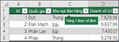
Freeze top row of heading:
When there are multiple rows, you can freeze the top row of the header column to scroll through the data only.
- Open Excel 2016.
- Make sure you have finished editing the box. To cancel Edit cells mode, press Enter or Esc.
- Select View> Freeze Top Row (in the Window group).
Save your workbook to OneDrive:
Save a workbook to OneDrive for Business or OneDrive (personal) to access the workbook from other devices and share and collaborate with others.
- Select File> Save As.
- To save to OneDrive for Business, select OneDrive – <Company name>.
- To save to OneDrive (personal), select OneDrive – Personal.
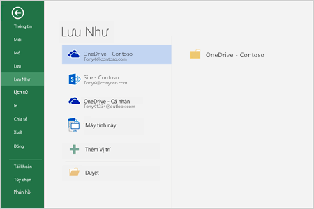
- Enter a name for the file, then select Save.
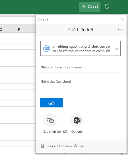
Share your workbook with others:
- Select Share on the ribbon. Or choose File > Share.
Note: If your file has not been saved to OneDrive, you will be prompted to upload the file to OneDrive for sharing.
- Select who you want to share from the drop-down menu or enter a name or email address.
- Add a message (optional), then select Send.
Leave a Reply